Open the LADCO Urban Increment R-Shiny App (updated)
App Description
The LADCO Urban Increment R-Shiny App displays the urban, rural, and urban increment PM2.5 concentrations for central counties in Core-Based Statistical Areas (CBSAs) across the lower 48 states. Users can select one or more states, one or more CBSAs in the selected states, and then one or more counties in the selected CBSAs to display stacked bar charts and tabulated urban increment data. Descriptions of the data and methods used to develop this tool follow.
This version of the app has been updated from the original app in several ways. (1) Urban areas are now defined based on CBSAs rather than land use classified as urban. This is computationally much faster. In the Great Lakes region, there is excellent overlap between the two definitions of urban areas. (2) Rural PM2.5 is averaged within a 150-mile radius of the CBSA rather than by state. These averages are more representative of the rural background around the urban area, and this approach more closely parallels EPA’s monitor-based approach (described below). (3) Urban increments are given for each county in an urban area rather than for the urban area as a whole. This provides more details about variation in the urban increment within urban areas. (4) Users can choose to display the urban increment based on the mean, 90th percentile, or maximum grid cell in the county.
Background
With the promulgation of a revised annual PM2.5 standard in February 2024 there is a demand for new air quality analysis products to understand the current profile of particulate pollution in the U.S. One of the data analysis products that contributes to the nonattainment area designations process is an urban increment analysis (see section 1.4 of US EPA, 2024). Per this memo, “the goal of the urban increment analysis is to estimate the local contribution to urban PM2.5 as measured at violating regulatory monitor sites and thereby provide additional evidence to consider in deciding which nearby areas with sources contributing to the monitored violations in the area to include within the boundary of the designated nonattainment area.”
The conventional approach for an urban increment analysis is to use surface monitors sited in urban and rural areas to estimate an urban increment at potential violating monitors. The urban monitors are part of the Chemical Speciation Network (CSN), and the rural PM2.5 concentrations are estimated using data from the IMPROVE program. The urban increment is simply the difference between a period-averaged concentration at the urban monitor and an analogous concentration at rural monitors that are within 150 miles of the urban site. Given the sparsity of the IMPROVE network, particularly in the Great Lakes region, there is an opportunity to explore alternative urban increment analyses that are based on PM2.5 data with more continuous spatial coverage.
Satellite PM2.5 Data
The Atmospheric Composition and Analysis Group at Washington University have developed satellite-derived global and regional PM2.5 data (Figure 1). These data are a fusion of satellite, modeled, and surface data. The fused data are estimated for “annual and monthly ground-level fine particulate matter (PM2.5) by combining Aerosol Optical Depth (AOD) retrievals from the NASA MODIS, MISR, SeaWIFS, and VIIRS with the GEOS-Chem chemical transport model, and subsequently calibrating to global ground-based observations using a residual Convolutional Neural Network (CNN).” The V6.GL.02.02 data are available for 1998-2022 on a 0.01 degree grid. Given the spatial continuity of these data and their relatively high correlation with surface observations, they provide a viable alternative to surface monitors for use in an urban increment analysis.
Methods
We used a GIS (ArcGIS Pro 3.3.2) to conduct all of the calculations and data processing steps for this analysis. The basic approach was to convert the netCDF gridded PM2.5 data to a raster, separate the raster into rural and urban PM2.5 rasters, and then use zonal statistics to get the concentrations in the rural and urban areas. Urban areas were defined as central counties within a metropolitan CBSA, and rural areas were defined as areas in the U.S. within 150 miles of a CBSA and outside an urban area. With the urban and rural concentrations, we could then calculate the urban increment in each urban county. Note that urban concentrations were calculated as either county means, 90th percentile values, or maxima. 90th percentile values are most likely to track concentrations at the controlling monitors. Additionally, the use of CBSAs to define urban areas should work well for most of the U.S. but will include vast rural areas in parts of the western U.S. where counties and their related CBSAs are very large. The detailed steps and data that we used are described below.
This app was developed by Zac Adelman and Angie Dickens at LADCO.
Data
- PM2.5 data: 2022 global 0.01 degree PM2.5 data in netCDF format (Washington University V6.GL.02.02)
- CBSA definitions: Census Core-Based Statistical Area (CBSA) to Federal Information Processing Series (FIPS) County Crosswalk (National Bureau of Economic Research, July 2023)
- U.S. Counties Map: USA Census Counties layer from the ESRI Living Atlas (dtl_cnty, accessed October 2024)
Processing Steps
- Use R to convert netCDF PM2.5 data to a raster and window in on the contiguous U.S. (download R code).
- Load the PM2.5 raster (Figure 1) and the CBSA County Crosswalk into ArcGIS Pro.
- Join the CBSA County Crosswalk table to the USA Counties map.
- Develop an urban areas (CBSAs) layer by selecting and deleting counties in the attribute table for the joined CBSA-Counties layer that: (a) are not in a CBSA, (b) are in a micropolitan CBSA, or (c) are in outlying counties of a CBSA. This will leave just central counties in a metropolitan CBSA (Figure 2).
- Develop a rural PM2.5 layer for areas in the counties layer but not in the urban areas layer (Figure 2).
- -Prepare to combine the layers:
- -Adjust the extents to match: Use Clip Raster to clip the counties and urban area (CBSA) rasters to the extent of the PM2.5 raster.
- -Handle missing data explicitly using Raster Calculator to specify that NoData points should be 0s.
- –Resample each raster to the PM2.5 raster to adjust grids so that they match exactly.
- -Combine the counties and urban area (CBSA) layers with the PM2.5 layer using Raster Calculator and the conditions that the adjusted urban areas layer = 0 (i.e., is not urban) and the adjusted counties layer = 1 (i.e., is in a U.S. county).
- -Prepare to combine the layers:
- Calculate the (a) mean, (b) 90th percentile, and (c) maximum PM2.5 within urban CBSA counties (Figure 3). This will calculate the concentration for each county. Use Zonal Statistics as Table to combine the PM2.5 layer with the urban areas (CBSA) layer and calculate the mean using statistics type = (a) Mean, (b) Percentile, with percentile set to 90, or (c) Maximum.
- Calculate the mean PM2.5 within rural areas within 150 miles of a CBSA (Figure 5).
- -Merge all counties in a CBSA into one polygon using Dissolve.
- -Apply a 150 mile buffer to this CBSA layer using the Buffer tool. You will have buffers for each CBSA (Figure 4).
- -Use Zonal Statistics as Table to combine the PM2.5 layer with the buffer layer and calculate the mean using statistics type = Mean. This step calculates the average PM2.5 in rural areas around each CBSA (Figure 5).
- Combine the urban and rural PM2.5 layers by joining the two attribute tables by CBSA. This will give you a layer with entries for each county, with the CBSA mean rural concentration and the county mean, 90th percentile, and maximum urban concentration.
- Calculate the urban increment by creating a new field in the attribute table of the new combined layer and using Calculate Field to subtract the rural mean PM2.5 from the urban mean/90th percentile/maximum PM2.5 (Figures 6-8). Figure 9 shows the 90th percentile urban increments zoomed in on and scaled to the Great Lakes region.
- Also calculate the mean/90th percentile/maximum PM2.5 for each CBSA as a whole using Zonal Statistics as Table.
Results
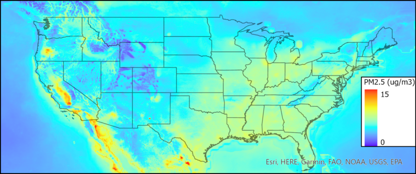
Figure 1. Washington University 0.01 degree 2022 average PM2.5.
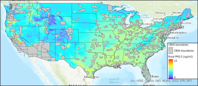
Figure 2. Metropolitan Core Based Statistical Areas (CBSAs, central counties only) and PM2.5 concentrations in rural areas in the U.S.
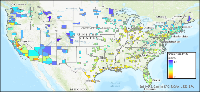
Figure 3. Mean PM2.5 for urban counties (central counties in metropolitan CBSAs).
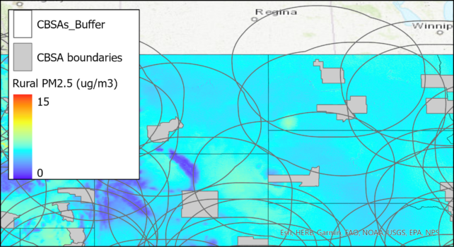
Figure 4. Metropolitan CBSA and rural PM2.5 with 150-mile buffers around CBSAs, zoomed in on the northern Great Plains region. The colored areas within each buffer were subsequently averaged to give the mean concentrations shown in Figure 5.
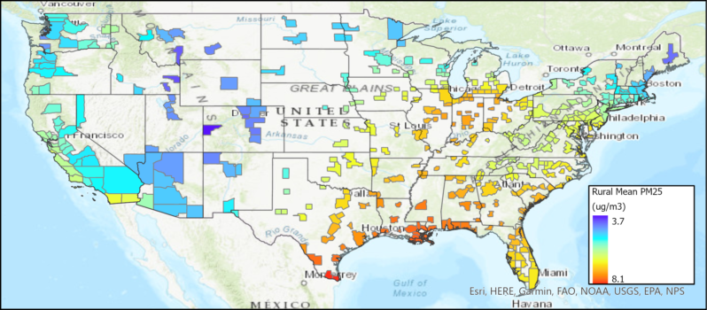
Figure 5. Mean PM2.5 for rural areas in the U.S. within 150 miles of each CBSA. Concentrations are given for each CBSA as a whole.
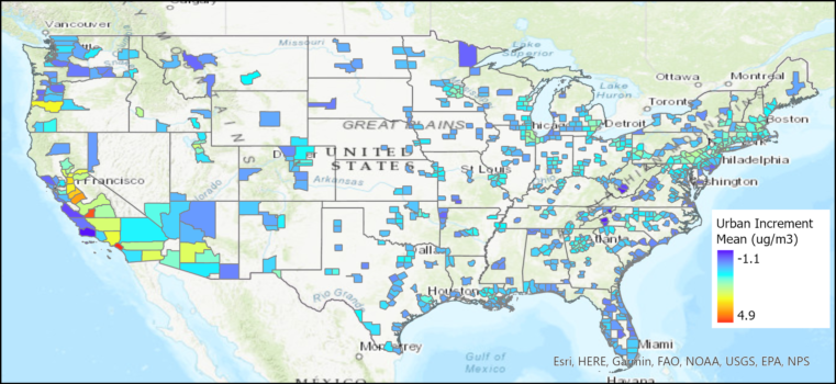
Figure 6. Urban increment based on the mean concentration for urban counties, determined as the difference between the mean urban and mean rural PM2.5 concentrations.
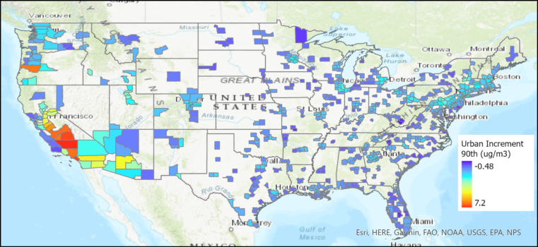
Figure 7. Urban increment based on the 90th percentile concentration for urban counties, determined as the difference between the 90th percentile urban and mean rural PM2.5 concentrations.
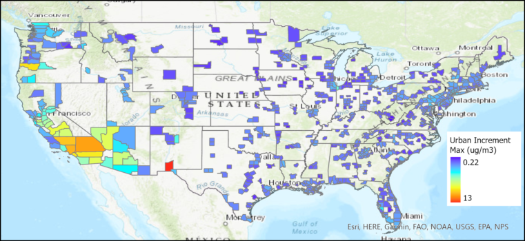
Figure 8. Urban increment based on the maximum concentration for urban counties, determined as the difference between the maximum urban and mean rural PM2.5 concentrations.
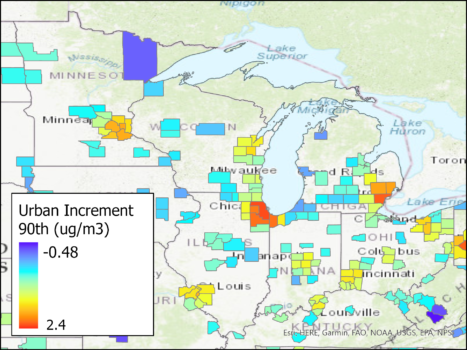
Figure 9. Urban increment based on the 90th percentile concentration for urban counties in the Great Lakes region.


